
“Wait a minute… why are there two identical names on this list?”
If you’ve ever found yourself double-checking rows in Excel and thinking, “Didn’t I already see this somewhere?”, you’re not alone.
Duplicates have a sneaky way of slipping into spreadsheets. If you’re working with lots of data, spotting them manually can feel like finding a needle in a haystack.
That’s where Excel’s built-in tools come to the rescue.
So, if you’re tracking sales data, managing a guest list, or updating inventory, learning how to highlight duplicates can save you tons of time and prevent mistakes.
In this guide, we’ll show you exactly how to do it, step by step.
Introduction
Excel offers powerful tools to manage and analyze data. One common task is identifying duplicate entries, which can be achieved through various methods, including built-in features and custom formulas. This guide will walk you through these methods with practical examples and visuals.
Highlighting Duplicates Using Built-in Conditional Formatting
Excel’s built-in conditional formatting feature allows you to quickly highlight duplicate values in a selected range.
1.Select the Range: Click and drag to select the cells where you want to check for duplicates.
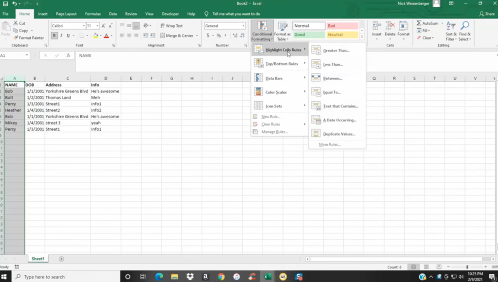
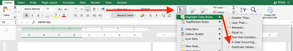
2.Navigate to Conditional Formatting:
o Go to the Home tab.
o Click on Conditional Formatting in the Styles group.
3.Choose Duplicate Values:
o Hover over Highlight Cells Rules.
o Click on Duplicate Values.
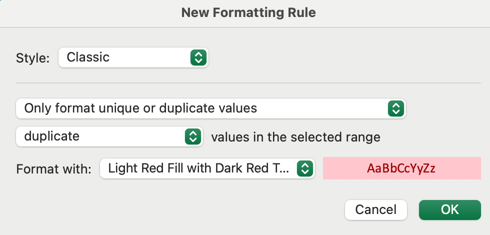
4.Set Formatting Options:
o In the dialogue box, choose the formatting style for duplicates.
o Click OK.
Highlighting Duplicates Without First Occurrences
Sometimes, you may want to highlight only the second and subsequent occurrences of duplicate values. This requires a custom formula.
1.Select the Range: Choose the cells to format.
2.Open New Formatting Rule:
o Go to Home > Conditional Formatting > New Rule.
3.Use a Formula:
o Select Use a formula to determine which cells to format.
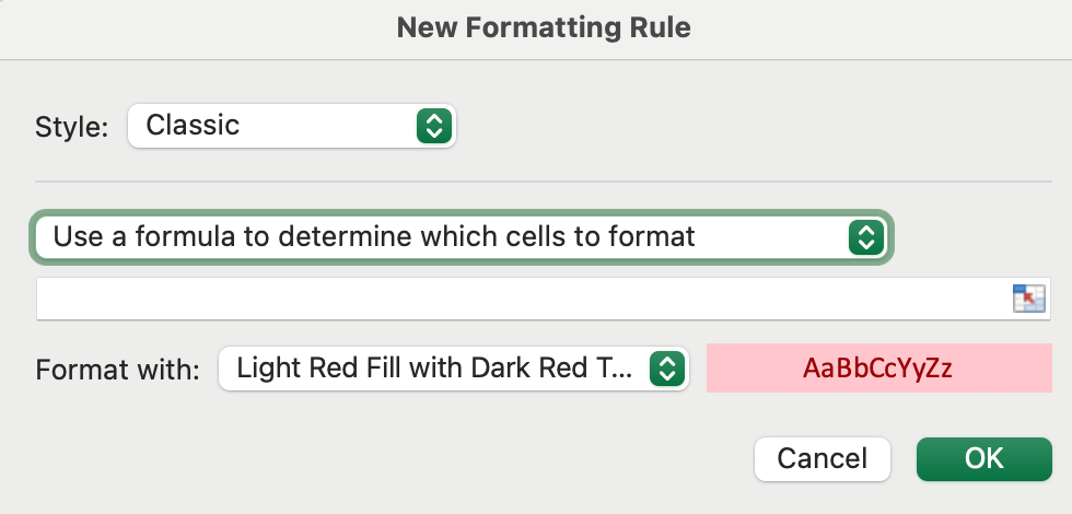
Enter the formula:=COUNTIF($A$2:$A2,A2)>1
4.Set Formatting:
o Click Format, choose your desired formatting, and click OK.
Enter the formula:=COUNTIF($A$2:$A2,A2)>1
4.Set Formatting:
oClick Format, choose your desired formatting, and click OK.
Highlighting Duplicates Across Multiple Columns
To find duplicates across multiple columns, you can use the COUNTIF function.
1.Select the Range: Highlight the range across multiple columns (e.g., A2:C8).
2.Open New Formatting Rule:
oGo to Home > Conditional Formatting > New Rule.
3.Use a Formula:
oSelect Use a formula to determine which cells to format.
=COUNTIF($A$2:$C$8,A2)>1
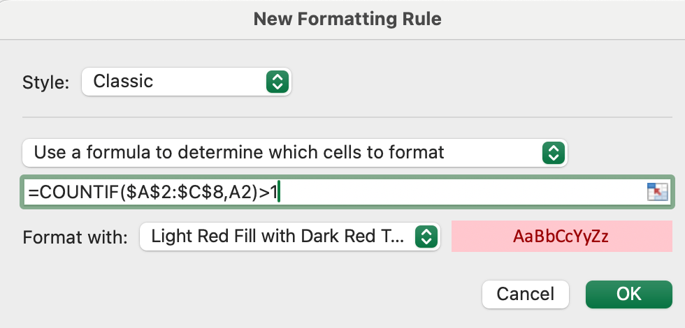
4.Set Formatting:
oClick Format, choose your desired formatting, and click OK.
Highlighting Entire Rows Based on Duplicate Values
To highlight entire rows where a specific column has duplicate values, use the COUNTIF function in a formula.
1.Select the Entire Data Range: For example, A2:D10.
2.Open New Formatting Rule:
oGo to Home > Conditional Formatting > New Rule.
3.Use a Formula:
oSelect Use a formula to determine which cells to format.
Enter the formula (assuming duplicates are in column A):To highlight duplicate rows excluding 1st occurrences:
=COUNTIF($A$2:$A2, $A2)>1

To highlight duplicate rows including 1st occurrences:
=COUNTIF($A$2:$A$10, $A2)>1
6.Set Formatting:
oClick Format, choose your desired formatting, and click OK.
Advanced Techniques – Highlighting Nth Occurrences
To highlight the Nth occurrence of a duplicate, modify the COUNTIF formula accordingly.
Example: Highlighting 3rd and Subsequent Occurrences
Use the Formula:=COUNTIF($A$2:$A2,A2)>=3
2. Apply Conditional Formatting:
Follow the same steps as before to set up a new formatting rule using this formula.
Common Issues and Troubleshooting
Issue 1 – Excel Highlights Unique Values as Duplicates
Cause: Excel may misinterpret numeric strings due to its 15-digit precision limit.
Solution: Prefix the values with an apostrophe (‘) to treat them as text.
Issue 2 – Conditional Formatting Not Working Across Entire Workbook
Cause: Conditional formatting rules are worksheet-specific.
Solution: Apply the formatting to each worksheet individually or use VBA for a workbook-wide solution.
FAQs
Q1: Can I highlight duplicates in non-adjacent columns?
A: Yes, but you’ll need to use a formula that references each specific column.
Q2: How do I remove duplicates after highlighting them?
A: Use the Remove Duplicates feature under the Data tab.
Q3: Can I highlight duplicates based on multiple criteria?
A: Yes, use the COUNTIFS function to set multiple conditions.
Conclusion
Keeping your data clean and error-free doesn’t have to be a headache.
When Excel’s powerful tools are available at your fingertips, spotting and highlighting duplicates is super quick. The key is to understand how to use the tools.
Now, whether you want to use the built-in features or craft custom formulas to highlight duplicates in Excel, you’ve got everything you need to take control of your data.
Mastering these techniques is a game-changer for keeping your spreadsheets sharp, accurate, and totally reliable
For a detailed visual tutorial, you can watch the following video: