

When working with wide spreadsheets in Excel, navigating data can quickly become frustrating. You scroll to the right to view details, but the column headers or reference data disappear. That’s where freezing columns in Excel comes in handy. This guide shows you all you need to know about freezing columns in Excel. No matter if you’re a beginner or experienced, we’ll cover the concept. We’ll provide step-by-step instructions, share real-life examples, and answer common questions.
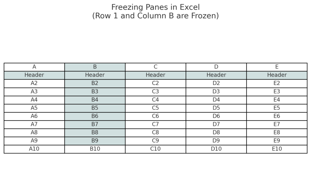
What Is Freezing in Excel?
Freezing in Excel locks certain rows or columns. This keeps them visible while you scroll through the sheet. It’s commonly used to:
- Keep headers visible while scrolling.
- Maintain important identifiers (like names, dates, or categories) on screen.
- Improve data readability in large spreadsheets.
When you freeze rows or columns in Excel, a solid line appears. This line is below the frozen row or to the right of the frozen column. It shows where the freeze is applied.
There are three types of freezing options in Excel:
- Freeze Top Row
- Freeze First Column
- Freeze Panes (Custom freezing for multiple columns and/or rows)
How to Freeze Multiple Columns in Excel
To freeze multiple columns, you’ll use the Freeze Panes option. Here’s how to do it step-by-step:
Step-by-Step Instructions to Freeze Multiple Columns
- Open your Excel worksheet.
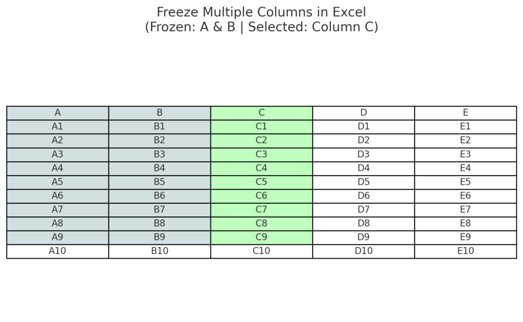
- Click the column to the right of the columns you want to freeze.
- For example, if you want to freeze Columns A and B, click on Column C.
- Go to the “View” tab in the Ribbon.
- In the “Window” group, click “Freeze Panes.”
- Select “Freeze Panes” from the dropdown menu.
Excel will insert a vertical line to the right of the frozen columns, locking Columns A and B in place.
Examples of Freezing Multiple Columns in Real Life
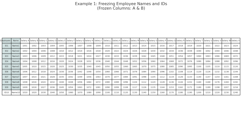
Example 1: Freezing Employee Names and IDs
You’re working on a payroll sheet with hundreds of employees. Freeze Columns A and B to keep names and IDs visible while scrolling. Salary data runs from Column C to Column Z.
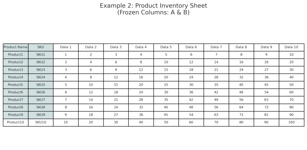
Example 2: Product Inventory Sheet
Your inventory list has product names in Column A and SKUs in Column B. It also includes many columns for dates, quantities, and stock levels. Freeze the first 2 columns so you always know which product you’re analyzing.
Example 3: Academic Scorecard
In a student scorecard:
- Columns A–D show student details: Roll No, Name, Class, and Section.
- Column E and beyond list subject marks.
Freezing Columns A–D helps you navigate the wide dataset. It keeps key identifiers visible.

Benefits of Freezing Multiple Columns in Excel
Freezing multiple columns provides several advantages, especially for large datasets. Below are key benefits explained in depth:
Improved Data Navigation
Scrolling through a large spreadsheet without freezing key columns can be disorienting. Freezing ensures essential labels or data remain visible as you move horizontally.
Example: Freezing the “Account Name” column in financial reports lets you easily match transactions. This is helpful, especially when looking at data on the far right.
Increased Data Accuracy
Freezing reference columns helps prevent mistakes. For example, it stops you from entering data in the wrong row or column.
Example: In data entry forms, freezing customer ID and name ensures data is linked correctly to the right customer.
Enhanced Productivity
Users work faster and more confidently because they don’t have to scroll back for context.
Example: While editing large marketing campaign reports, keeping campaign names frozen improves task flow.
Better Decision Making
For managers and analysts, seeing key identifiers helps them quickly spot patterns, trends, or outliers.
Example: While reviewing KPI dashboards, frozen departments or regions give quick comparative insights.
Simplifies Collaboration
Frozen panes help teams understand shared data better. This is especially true for members who are not used to the dataset’s layout.
Example: Shared sales sheets with frozen rep names prevent confusion during team performance reviews.
HOW TO FREEZE MULTIPLE ROWS AND COLUMNS (EASY 2-STEP METHOD)
Frequently Asked Questions (FAQ’s)
Can I freeze non-adjacent columns in Excel?
No. Excel only allows freezing adjacent columns from the left side. To highlight non-adjacent data, try using “New Window” or changing your sheet’s layout.
Why can’t I see the freeze option?
Make sure you’re on the “View” tab. If your worksheet is protected or in “Page Layout” view, the “Freeze Panes” option may be disabled. Switch to “Normal View.”
How do I unfreeze columns?
- Go to the View tab.
- Click Freeze Panes.
- Select Unfreeze Panes.
This will remove all frozen rows and columns.
Can I freeze both rows and columns at once?
Yes. Use “Freeze Panes” by selecting a cell below the rows and to the right of the columns you want to freeze.
Example: To freeze Rows 1–2 and Columns A–B, select cell C3 and click “Freeze Panes.”
Is there a keyboard shortcut to freeze columns?
There is no default shortcut, but you can press Alt + W + F + F in sequence to apply Freeze Panes.
Conclusion
Freezing multiple columns in Excel is a simple but effective feature. It makes working with large datasets much easier. Keeping key columns visible boosts productivity, accuracy, and clarity. This matters whether you track employee records, analyze financial data, or manage inventory. Follow the steps and examples above to master this skill with confidence.