

Excel is great for crunching numbers. It’s also helpful for formatting data visually. A useful but often overlooked feature is strikethrough formatting. You can easily cross out text. The strikethrough feature helps keep spreadsheets organized. You can mark tasks as complete, show outdated info, or track changes without deleting data. This makes it easier to understand your work. In this guide, you’ll discover how to cross out text in Excel. We’ll cover methods, examples, benefits, and common FAQs.
What Is Cross Out Text in Excel?
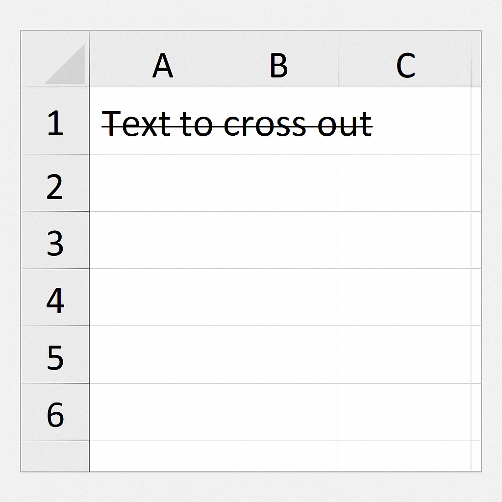
Crossing out text in Excel means adding a line through the middle of the cell’s content. This is often called strikethrough. It’s a formatting option that indicates when something is done, canceled, or inactive. It also keeps the original data.
Here’s how it looks:
Before: Buy Office Chair After: Buy Office Chair
The text remains intact, but it’s visually shown as “crossed out.”
How to Cross Out Text in Excel
You can apply strikethrough formatting in Excel in a few ways. You can do it manually, use keyboard shortcuts, or set it up with conditional formatting.
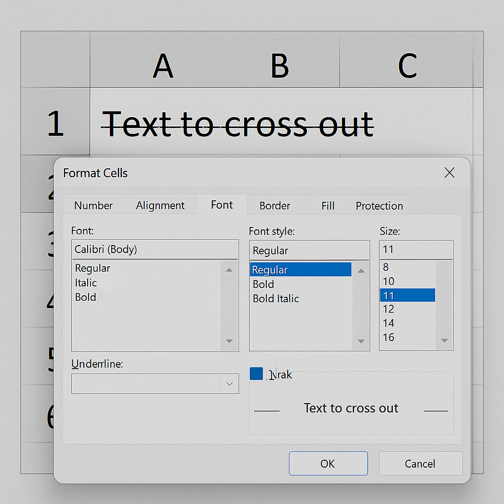
Method 1: Use Format Cells Dialog
This is the most straightforward method for applying strikethrough.
Steps:
- Select the cell(s) or text you want to cross out.
- Right-click and choose Format Cells.
- In the dialog box, go to the Font tab.
- Check the box labeled Strikethrough.
- Click OK.
Works well for static formatting.
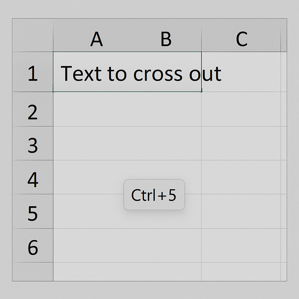
Method 2: Use Keyboard Shortcut
For faster formatting, use a quick shortcut.
Windows:
Ctrl + 5
Mac:
Command (⌘) + Shift + X
Just select the text or cell and press the keys — the strikethrough formatting will toggle on/off.
Method 3: Use the Excel Ribbon (Customizable)
Excel doesn’t show the strikethrough icon by default, but you can add it.
Steps to Add Strikethrough to Ribbon or Toolbar:
- Click File > Options.
- Go to Quick Access Toolbar.
- From the left panel, select All Commands.
- Find and add Strikethrough to your toolbar.
- Click OK.
Now you can apply strikethrough with a single click.
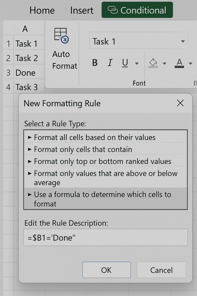
Method 4: Apply Strikethrough with Conditional Formatting
Use this if you want Excel to automatically cross out text based on a condition (e.g., when a task is marked as complete).
Example Scenario:
Column A = Task Name Column B = Status (e.g., “Done”)
Steps:
- Select the range in Column A.
- Go to Home > Conditional Formatting > New Rule.
- Choose “Use a formula to determine which cells to format.”
- Enter a formula like:
=$B1=”Done”
- Click Format, go to Font, and check Strikethrough.
- Click OK.
Now, when you mark a task as “Done” in Column B, the corresponding task in Column A will be automatically crossed out.
Examples of Crossed Out Text in Excel
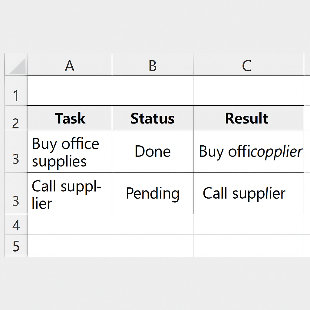
Example 1: To-Do List
| Task | Status | Result |
| Buy office supplies | Done | Buy office supplies |
| Call supplier | Pending | Call supplier |
Used with conditional formatting.
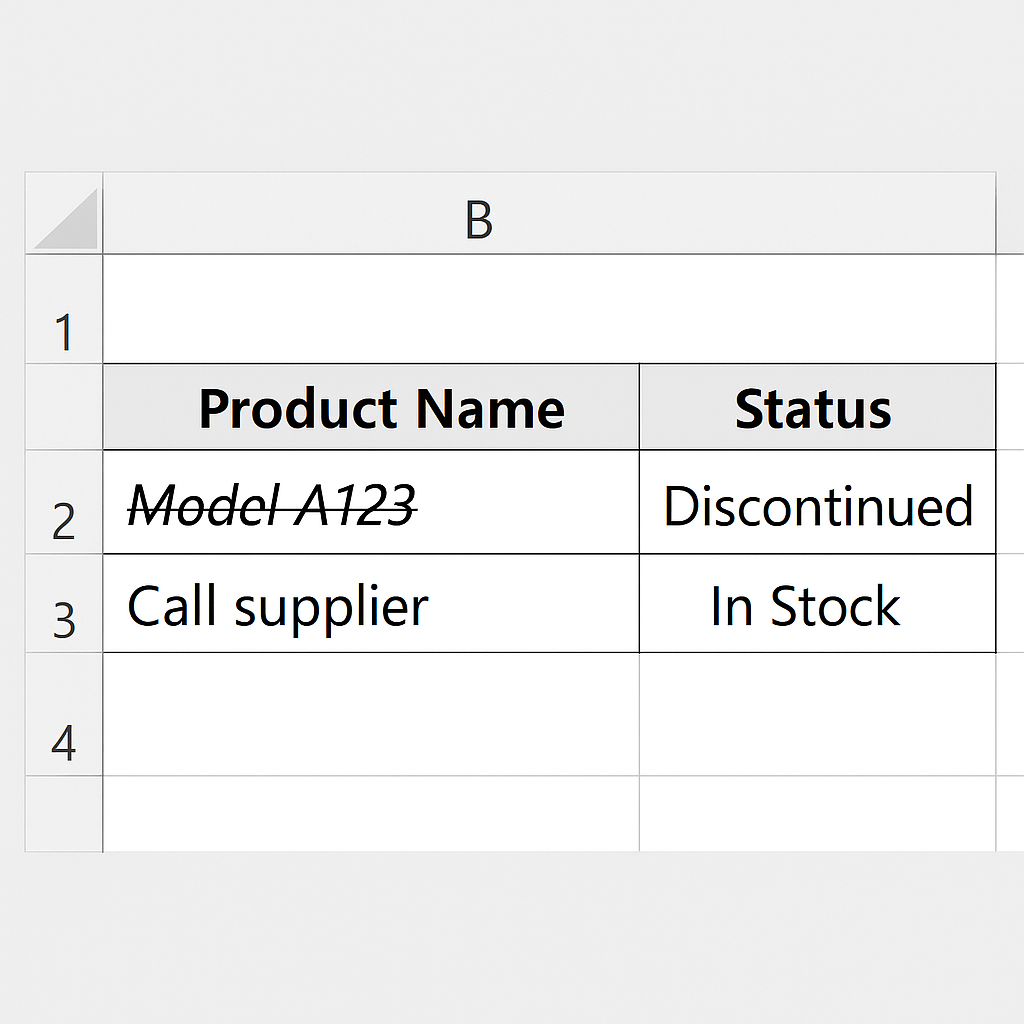
Example 2: Canceled Products in Inventory
| Product Name | Status |
| Model A123 | Discontinued |
| Model B456 | In Stock |
Here, discontinued items are crossed out to avoid confusion while keeping data visible.
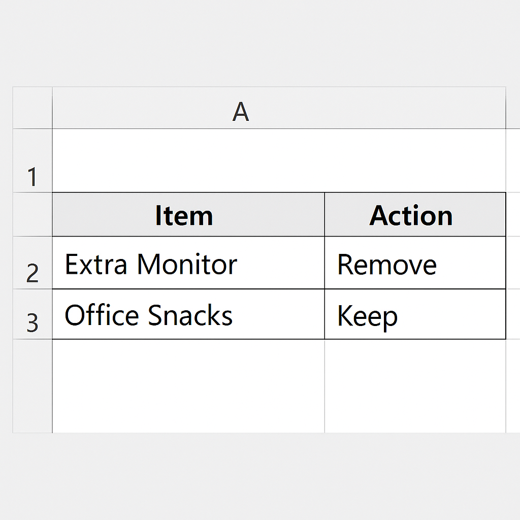
Example 3: Budget Planning
| Item | Action |
| Extra Monitor | Remove |
| Office Snacks | Keep |
This makes it easy to show changes while maintaining transparency.
Benefits of Using Cross Out Text in Excel
Visual Task Tracking
Strikethrough helps you track completed tasks without deleting them. This is essential for:
- Project management
- Daily to-do lists
- Client deliverables
Rather than deleting completed items, you separate them visually. This way, you can easily see what’s done and what’s still pending.
Preserves Data Transparency
Crossing out a value allows readers to see historical information. In business reporting or budgeting, this maintains transparency and ensures:
- Accountability
- Audit readiness
- Version comparison
You can display canceled orders, rejected expenses, or removed features. This way, you keep a record of the past.
Enhances Collaboration
When working in a team, you can strike through data to show changes. This way, nothing gets deleted, and collaboration becomes easier. Everyone can:
- See what was changed
- Understand why
- Restore values if needed
Saves Time on Reformatting
Strikethrough gives quick visual meaning. This cuts down on extra formatting and complexity. You don’t need a separate column for status or notes.
Useful for Dynamic Formatting
Conditional formatting with strikethrough lets Excel style data automatically using rules. This feature is great for dashboards, data validation, and smart tables.
Example:
- Cross out overdue items
- Strike through completed orders
- Hide duplicates visually
Applying Strikethrough in Excel
FAQ’s – Cross Out Text in Excel
Is strikethrough available in all Excel versions?
Yes, strikethrough is available in Excel 2010 and later for both Windows and macOS.
Can I cross out just part of the text in a cell?
Yes. Double-click the cell. Select the text you want. Then, apply strikethrough by pressing Ctrl + 5 or using Format Cells.
Can I remove strikethrough from text?
Absolutely. Repeat the steps using the shortcut or format menu. Then, uncheck or toggle off the strikethrough option.
Does strikethrough affect calculations?
No. Strikethrough is purely visual. The underlying value remains unchanged and can still be used in formulas.
Can I apply strikethrough with Excel Online?
Yes, Excel for the web supports strikethrough. Use:
- Ctrl + 5 (Windows)
- Format > Strikethrough from the ribbon
Conclusion
Crossing out text in Excel might seem small, but it’s a powerful tool when used wisely. Strikethrough formatting helps clarify information in task lists, inventory, and shared reports. It keeps the context while showing what has changed. This guide showed different ways to use it. We covered simple shortcuts and dynamic conditional formatting. Real-life examples and clear benefits were also included. Using strikethrough smartly can make your spreadsheets more readable, transparent, and efficient.