

Excel is a powerful tool used worldwide for organizing, analyzing, and visualizing data. One of its standout features is the ability to enhance readability through highlighting. Highlighting every other row, or banding, helps make large data sets easier to read. It adds clarity and lowers mistakes. In this guide, we’ll cover what highlighting is. We’ll give step-by-step instructions to highlight every other row in Excel. You’ll also find practical examples and the key benefits of this technique.
What is Highlight in Excel?
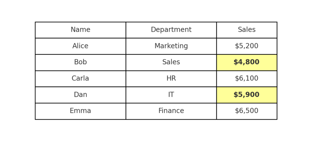
Highlighting in Excel means changing the format of certain cells, rows, or columns. You can use colors or shading. This helps draw attention to important data and makes the dataset look better and easier to read. Using alternating colors for rows helps users see data better. It cuts down on visual strain and boosts productivity.
How to Highlight Every Other Row in Excel
Highlighting every other row in Excel is straightforward, especially using Conditional Formatting. Here’s how you can easily do it:
Step 1: Select Your Data
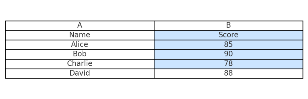
First, open your Excel workbook and select the range of cells you want to format.
Step 2: Go to Conditional Formatting
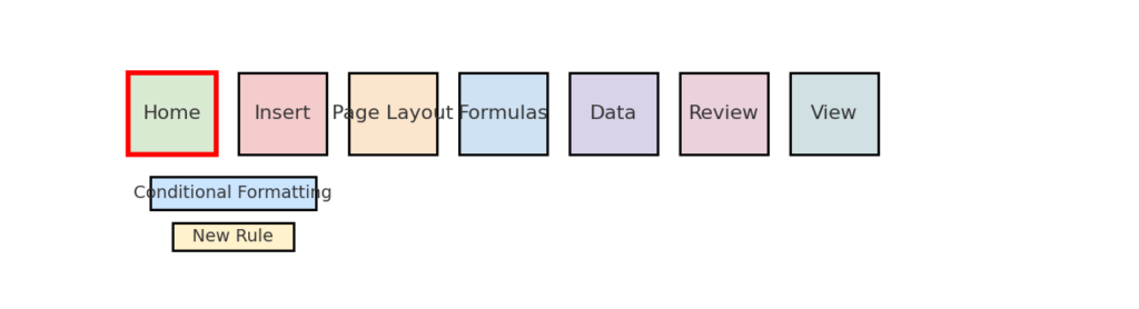
On the Excel ribbon, navigate to:
Home Tab > Conditional Formatting > New Rule.
Step 3: Create a New Rule
In the “New Formatting Rule” dialog box, select:
“Use a formula to determine which cells to format.”
Step 4: Enter the Formula
In the formula box, enter:
=MOD(ROW(),2)=0
This formula tells Excel to format every second row (even rows).
Step 5: Choose Formatting
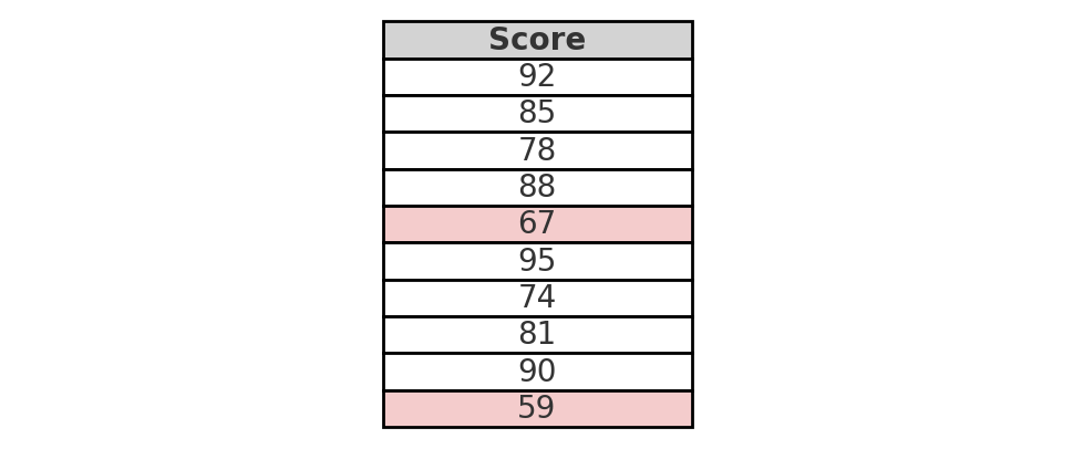
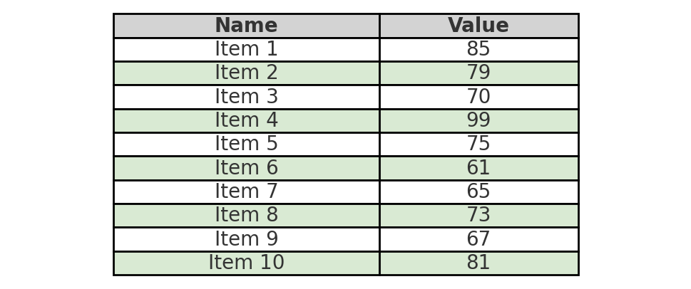
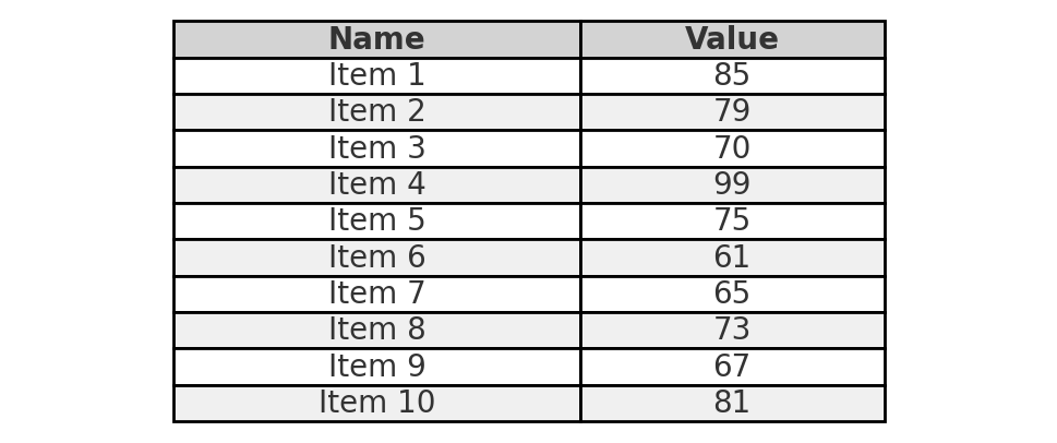
Click “Format” to set the desired fill color or pattern. Typically, a light grey or pastel shade works best.
Step 6: Apply the Rule
Click “OK” twice. Excel will immediately highlight every other row.
Practical Examples
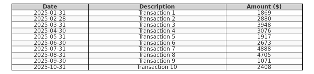
Example 1: Financial Reports
Imagine managing a financial report with hundreds of rows. Highlighting every other row makes the report clearer. This change cuts down on input errors and speeds up data analysis.
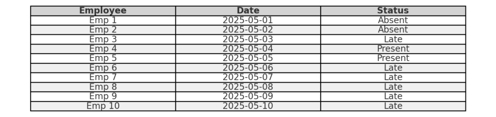
Example 2: Employee Attendance Sheets
Using alternating row colors on attendance sheets helps spot issues fast. You can easily see absences or strange timings. This improves payroll and HR accuracy.
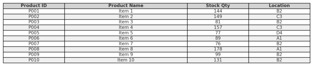
Example 3: Inventory Management
Inventory sheets can be cumbersome to read when containing multiple product lines. Highlighting alternate rows facilitates quick scanning and significantly reduces miscounting or overlooking items.
Benefits of Highlighting Every Other Row in Excel
Highlighting alternate rows in Excel has many benefits beyond just looking good. Here’s an in-depth look at these benefits:
Improved Readability
Using alternating colors helps reduce eye fatigue. This is especially true when looking at large data sets for a long time. This improved readability ensures that users can scan and interpret information more efficiently.
Enhanced Data Accuracy
Clear visual distinction minimizes mistakes like data misinterpretation or duplication. Accuracy is especially important for financial records, inventory tracking, and key business reports.
Time Efficiency
Quickly identifying data rows leads to faster decisions and better data handling. This boost in speed helps improve productivity and operations.
Professional Presentation
Visually appealing spreadsheets appear more professional and organized. Highlighting every other row can improve your reports. This makes them better for meetings, presentations, and official documents.
Better Focus
Highlighted rows grab the user’s attention. They cut down distractions and help focus on important data.
Highlight Every Other Row in Excel in 90 Seconds!
FAQ’s
Can I highlight every third or fourth row instead of every second row?
Yes, modify the MOD formula accordingly. For instance, use =MOD(ROW(),3)=0 for every third row.
Will the highlighting automatically adjust if new rows are inserted?
Yes, Excel’s conditional formatting changes the highlighting when you add, delete, or move rows in the formatted range.
Can I apply alternate row highlighting to columns as well?
Certainly! To highlight alternate columns, use the formula =MOD(COLUMN(),2)=0 instead.
Does highlighting affect Excel’s performance?
Basic conditional formatting, such as alternating row colors, doesn’t greatly affect Excel’s performance. However, extensive conditional formatting can slow Excel down slightly.
Conclusion
Highlighting every other row in Excel makes data easier to read. It helps reduce mistakes and boosts productivity. Using Excel’s conditional formatting tool to shade alternate rows is simple and useful. It’s a great tip for professionals working with large data sets. Using this simple visual strategy helps you manage data better. It keeps your reports professional and accurate. These traits are key in today’s data-focused world.