

Working with big datasets in Excel can be tough. It’s annoying when column headers or row labels scroll out of sight. That’s where freezing panes comes in handy. It helps you lock specific parts of your spreadsheet in place while you scroll through the rest. But what if you need to freeze both rows and columns simultaneously—i.e., freeze multiple panes? The good news is: Excel makes this possible with just a few clicks. In this guide, you’ll learn about multiple panes, how to freeze them in Excel, real-life examples, and their benefits.
What is Multiple Panes?
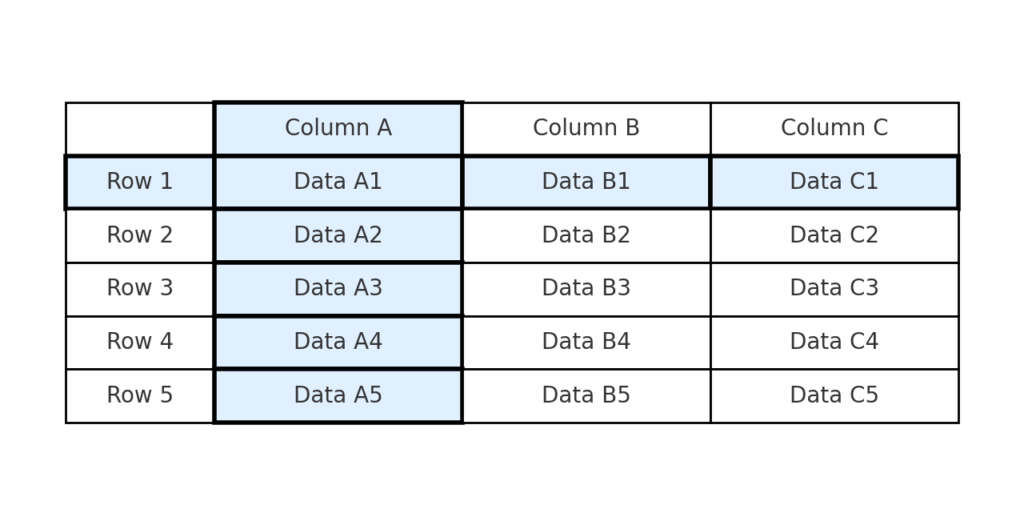
In Excel, the term pane refers to a section of a worksheet. When you freeze panes, you lock rows, columns, or both. This keeps them visible as you scroll through your spreadsheet.
Multiple panes means:
Freezing both:
- One or more rows from the top
- One or more columns from the left
This helps when your spreadsheet has row headers, like names, and column headers, like months. You want to keep both visible while you navigate.
How to Freeze Multiple Panes in Excel
To freeze multiple panes, select a cell and use the Freeze Panes option in Excel. Here are the detailed steps:
Step 1: Open Your Worksheet
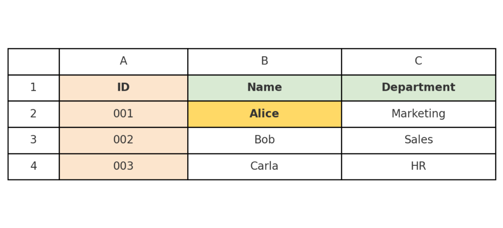
Open your Excel file that contains a large dataset. Label your header row and column clearly. For example, the top row should have field names, and the first column should include IDs or names.
Step 2: Identify the Cell Where You Want to Freeze Panes
To freeze rows and columns, select the cell below the rows and to the right of the columns you want to freeze.
Example:
If you want to freeze:
- Row 1 (headers)
- Column A (labels)
You need to click on cell B2 (row 2, column B).
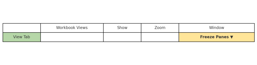
Step 3: Go to the View Tab
- Click on the View tab in the ribbon.
- Click Freeze Panes in the Window group.
- Select Freeze Panes from the dropdown menu.
Excel will freeze everything above and to the left of your selected cell. Now when you scroll vertically, Row 1 remains visible. When you scroll horizontally, Column A stays locked.
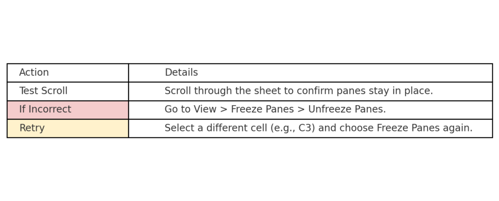
Step 4: Test and Adjust
Scroll through your sheet to ensure the right panes are frozen. If not:
- Go to View > Freeze Panes > Unfreeze Panes
- Try selecting a different cell and repeat
Excel allows only one freeze operation at a time. You cannot freeze two non-contiguous sections.
Examples of Freezing Multiple Panes in Excel
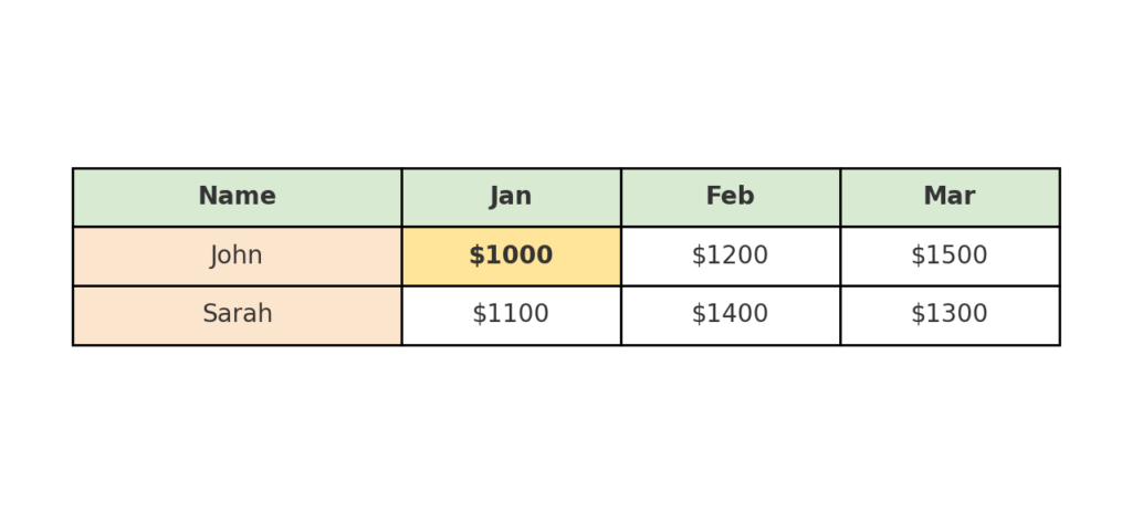
Example 1: Freezing Employee Names and Monthly Data Headers
| A | B | C | D |
| Name | Jan | Feb | Mar |
| John | $1000 | $1200 | $1500 |
| Sarah | $1100 | $1400 | $1300 |
Goal: Keep “Name” (Column A) and the months (Row 1) always visible. Action: Select cell B2, then click View > Freeze Panes > Freeze Panes.
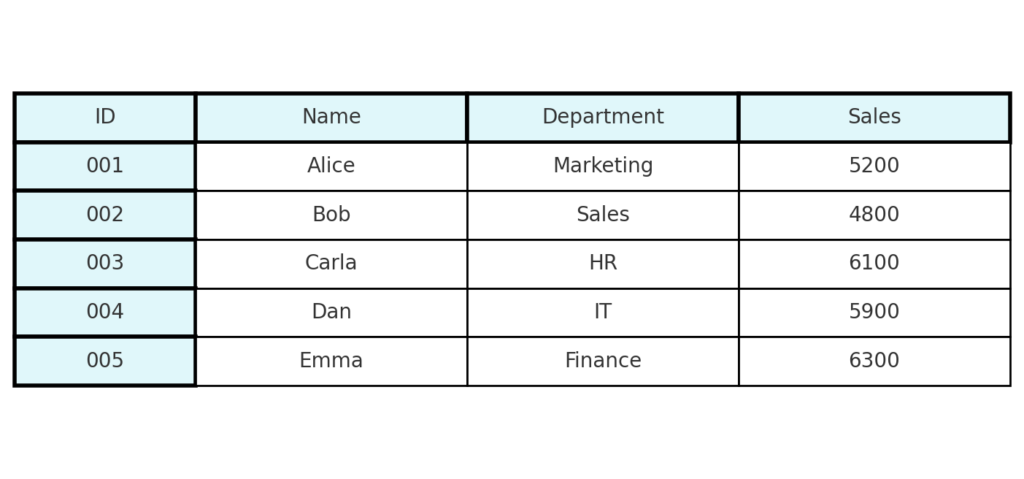
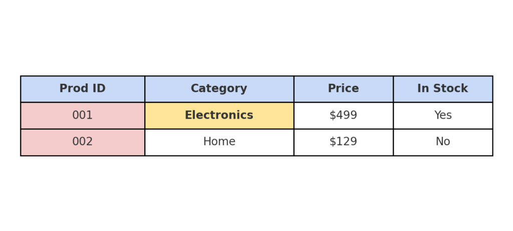
Example 2: Freezing Product IDs and Categories
| A | B | C | D |
| Prod ID | Category | Price | In Stock |
| 001 | Electronics | $499 | Yes |
| 002 | Home | $129 | No |
Goal: Keep column A and the top row visible while scrolling.
Action: Select cell B2, apply Freeze Panes.
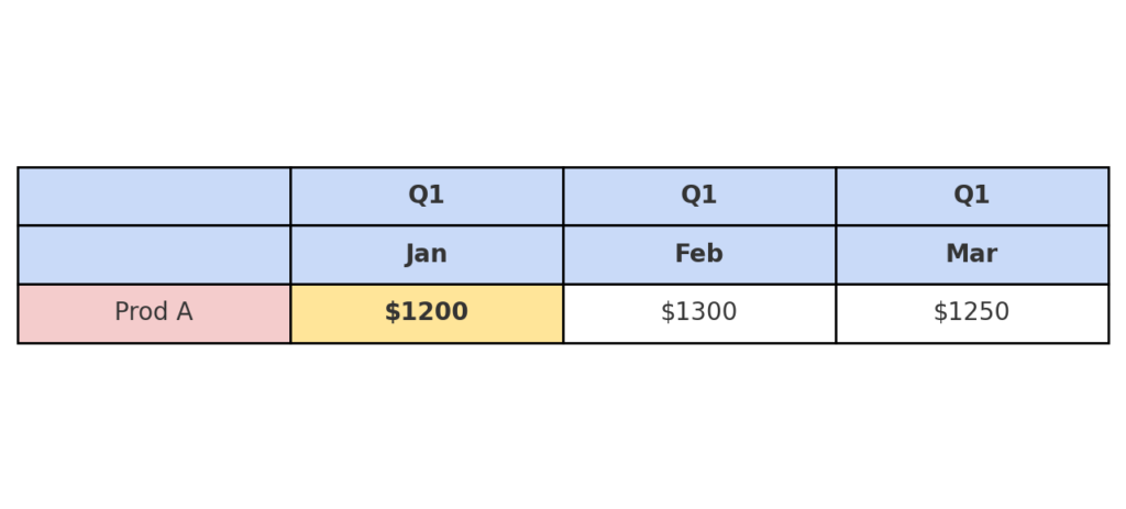
Example 3: Freezing Multi-Row Headers with Sidebar
| A | B | C | D |
| Q1 | Q1 | Q1 | |
| Jan | Feb | Mar | |
| Prod A | $1200 | $1300 | $1250 |
Goal: Freeze both Rows 1–2 and Column A.
Action: Select cell B3, then apply Freeze Panes.
Benefits of Freezing Multiple Panes in Excel
Keeps Headers Always in View
When working with long datasets, scrolling down causes headers to disappear. Freezing the top row helps you always know what data you’re viewing. Locking the first column keeps important details, like names or IDs, in view.
Improves Data Accuracy During Entry
Losing track of headers while entering data in many rows and columns can lead to mistakes. You might place values in the wrong cells. Locking headers helps you enter the right data in the correct column. This is essential in tasks like budgeting, attendance tracking, and inventory updates.
Saves Time in Large Workbooks
Freezing panes lets you work smoothly without scrolling back to check headers or names. This makes the workflow more efficient, especially for large spreadsheets with over 50 columns or thousands of rows.
Enhances Presentation and Reporting
Frozen panes help stakeholders, clients, and managers understand data better in spreadsheets. They can scroll freely and still understand the context of each value. This is especially important in financial models, performance dashboards, and project tracking templates.
Makes Collaboration Easier
Frozen panes in shared files or during Zoom presentations help everyone keep up. They show what each row or column means, so no one has to guess. This increases clarity and reduces the chance of miscommunication.
Compatible with Print Titles
When preparing to print your spreadsheet, frozen panes correspond with print titles. This ensures headers are repeated on each page—improving document readability and professionalism.
HOW TO FREEZE MULTIPLE ROWS AND COLUMNS (EASY 2-STEP METHOD)
FAQ’s
Can I freeze non-adjacent rows and columns?
No. Excel allows you to freeze only the rows above and columns to the left of your selected cell. Freezing multiple non-contiguous sections is not supported.
Does freezing panes affect printing?
No, frozen panes are only for on-screen navigation. To repeat headers on each printed page, go to Page Layout > Print Titles.
Is it possible to freeze panes in protected sheets?
You must unprotect the sheet before applying or modifying freeze panes. Once applied, you can re-protect the sheet as needed.
Conclusion
Freezing multiple panes in Excel is a great tool. It helps you see, navigate, and work accurately with large or complex datasets. Whether you’re working on sales reports, financial projections, or team performance sheets, this feature keeps your headers and labels visible while you scroll.