

Using large spreadsheets in Excel can feel overwhelming. You often scroll through rows and columns, losing track of headers or key identifiers. That’s where Excel’s Freeze Panes feature becomes a game-changer. You can keep certain rows or columns visible on your screen while you scroll. This makes it easier to see and use your data. In this guide, you’ll discover how to freeze rows and columns in Excel. You’ll learn to freeze the top row and the first column. We’ll cover real-world examples, step-by-step instructions, benefits, and answers to common questions.
What are Freezing Rows and Columns?
Freezing rows and columns in Excel helps keep important parts of your worksheet in view. This way, you can scroll through your data without losing sight of them.
- Freezing the top row keeps your header row visible when scrolling down.
- Freezing the first column locks the first column in place as you scroll right.
- You can freeze both simultaneously to keep row titles and column labels always on view.
This function doesn’t change data or formulas. It only changes how your worksheet appears on screen. This feature is helpful for navigating large datasets.
How to Freeze Top Row and First Column in Excel
Microsoft Excel provides multiple options under the View tab to manage freeze panes. Here’s how you can freeze both the top row and the first column together or individually:
Method 1: Freeze Top Row and First Column Simultaneously
Step-by-Step Instructions:
- Open your Excel worksheet.
- Click on the View tab in the ribbon.
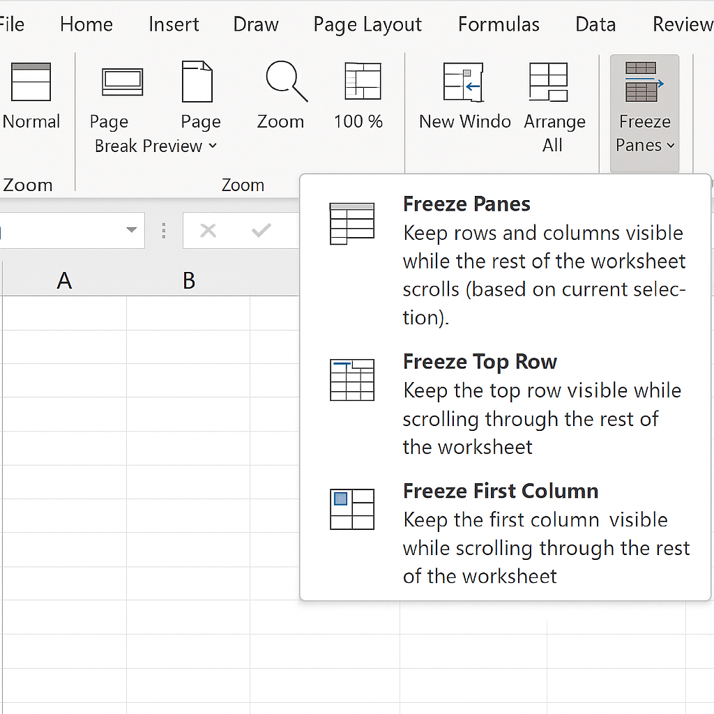
- Select Freeze Panes from the “Window” group dropdown.
- Choose Freeze Panes again (the first option in the dropdown).
Important: First, click the cell below the row and to the right of the column you want to freeze. For freezing the top row and the first column, click cell B2. This will lock the top row and the first column. They will stay visible while you scroll up and down or side to side.
Method 2: Freeze Top Row Only
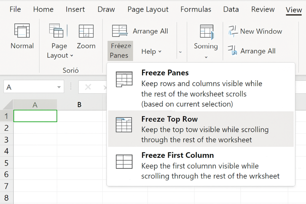
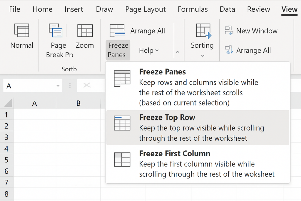
- Go to the View tab.
- Click on Freeze Panes.
- Select Freeze Top Row.
Now your header row (Row 1) will stay in place while you scroll downward.
Method 3: Freeze First Column Only
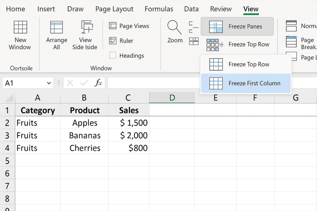
- Click the View tab.
- Select Freeze Panes.
- Choose Freeze First Column.
Your first column (Column A) will now remain visible as you scroll to the right.
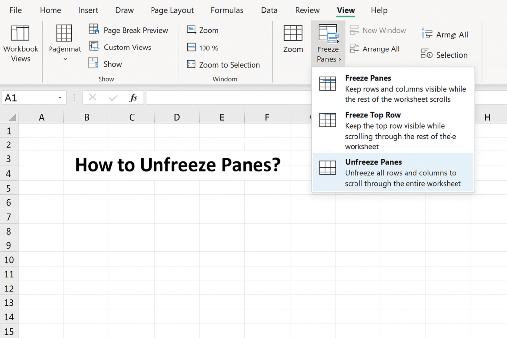
How to Unfreeze Panes?
If you want to remove freezing:
Go to View > Freeze Panes > Unfreeze Panes.
This will reset the view to default, allowing all rows and columns to scroll freely.
Examples
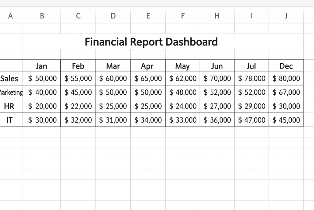
Example 1: Financial Report Dashboard
Picture a financial spreadsheet. The months are at the top (Row 1), and the departments are listed along the side (Column A). Freeze the top row and first column. This way, you can scroll through the revenue data and always see the department name and the month.
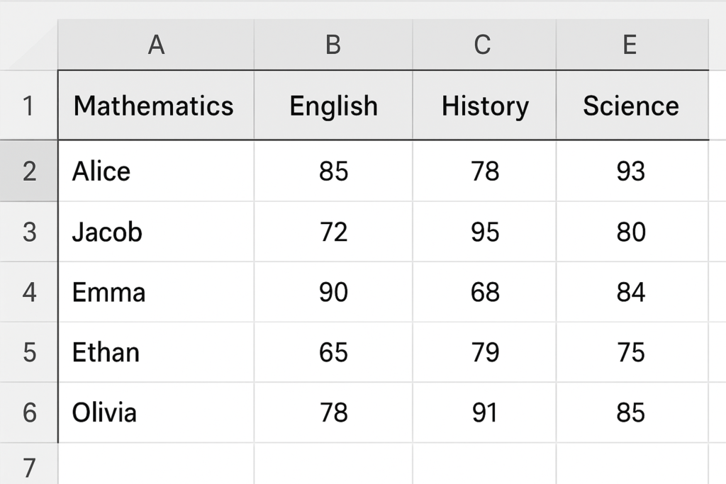
Example 2: Academic Performance Sheet
In a student gradebook, Row 1 contains subject names and Column A has student names. Freezing helps keep student names and subject headers visible. This makes it easy to analyze grades for different students and subjects.
Benefits of Freezing Rows and Columns in Excel
Enhanced Data Navigation
Freezing panes lets you scroll through large datasets. It keeps important context, like headers and labels, visible. This is vital for accuracy when reading long lists of information. Frozen headers in sales reports help you know what the data means. This is especially useful with hundreds of products and months.
Improves Readability and Reduces Errors
Keeping row and column identifiers visible helps you avoid reading data from the wrong spot. This is especially important in finance, HR, and legal records where precision is key.
Professional-Looking Workbooks
Clients, managers, and collaborators appreciate well-organized Excel sheets. A frozen header row and category column make the interface neat and easy to use. This setup helps users understand and present the information better.
Saves Time and Increases Productivity
Instead of scrolling back to the top or left to check a value, users can keep working smoothly. This small feature can save hours over the lifetime of a large project.
Supports Better Printing Layouts
To print the worksheet, freeze panes and set print options. This helps align the data correctly. Freeze panes aren’t visible in printouts. However, they help organize pages clearly on-screen.
How to Freeze the Top Row and First Column in Microsoft Excel ��[SPREADHSEET TIPS!]
FAQ’s
Is there a shortcut key to freeze top row in Excel?
While there’s no single-key shortcut, you can press Alt + W, F, R in sequence to freeze the top row. For freezing the first column, press Alt + W, F, C.
Does freeze panes work on Excel Online?
Yes, Excel Online supports freezing rows and columns. However, some features may be limited compared to the desktop version. The process is similar: go to View and use the Freeze Panes option.
How do I know if the row or column is frozen?
Excel visually shows a dark gray line just beneath the frozen row or beside the frozen column. If you scroll and the row or column stays fixed, freezing is active.
Can I freeze panes and also split windows in Excel?
Yes, but they are separate features. Freeze panes keeps part of the sheet visible while scrolling. Split divides the window into two or more scrollable areas. You can use both for advanced viewing setups.
Conclusion
Mastering the Freeze Panes feature in Excel helps you navigate spreadsheets easily. This is especially important when working with large data sets. Freezing the top row and first column keeps key labels and headers visible. This helps you understand data better, reduces errors, and speeds up your workflow. Freezing rows and columns makes your spreadsheets much easier to use. This skill helps with financial sheets, academic reports, inventory logs, and team dashboards. It doesn’t require formulas, coding, or complex tools—just a few clicks under the View tab.