

Summarizing a column in Excel is key when handling large datasets. It helps with clarity, decision-making, and reporting. When you analyze sales, manage budgets, or track performance, summarizing column data helps. It provides quick insights into totals, averages, counts, and more. You won’t need to scroll through every row. This guide covers what column summarization is and how to do it. You’ll learn to use built-in functions and tools. We provide real-life examples, a full list of benefits, and answers to common questions.
What is Summarizing a Column?
Summarizing a column in Excel means finding a key value or values that reflect the data in that column. Summarization gives you quick metrics instead of looking at each row one by one, like:
- Total (using SUM)
- Average (using AVERAGE)
- Minimum and Maximum
- Count of entries
- Frequency of unique values
- Conditional summaries (using SUMIF, COUNTIF, AVERAGEIF)
- Aggregated values through PivotTables or Subtotals
These summaries show trends, outliers, and key metrics. They make your data easier to understand and report.
How to Summarize a Column in Excel
You can summarize a column in Excel in different ways. It depends on the type of summary you want and how your data is set up.
Method 1: Use Basic Summary Functions
The most direct way to summarize a column is by applying built-in Excel functions:
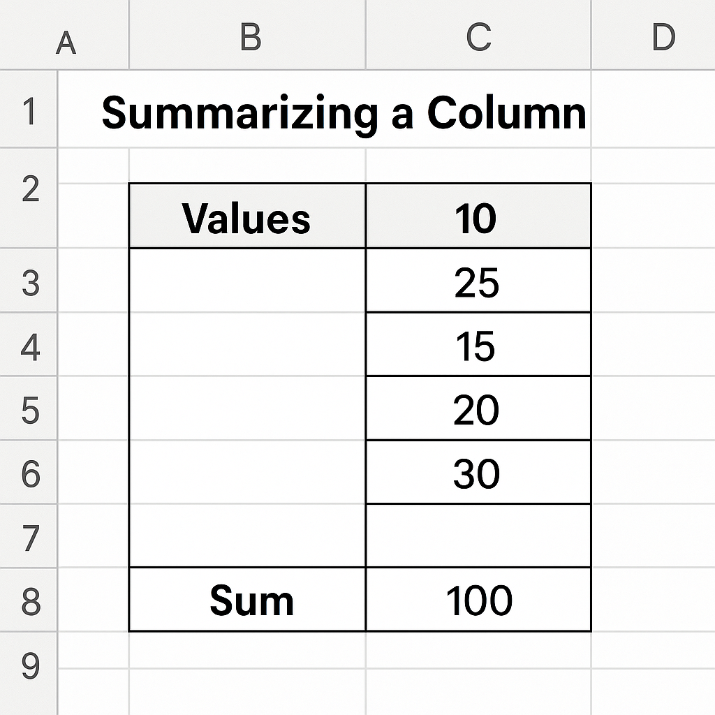
SUM
To get the total of all numeric values in a column:
=SUM(A2:A100)
This adds all the values from cell A2 to A100.
AVERAGE
To find the average of a column:
=AVERAGE(A2:A100)
COUNT
To count how many numeric values exist in a column:
=COUNT(A2:A100)
If you want to count all non-blank entries (including text):
=COUNTA(A2:A100)
MAX and MIN
To get the highest and lowest values:
=MAX(A2:A100) =MIN(A2:A100)
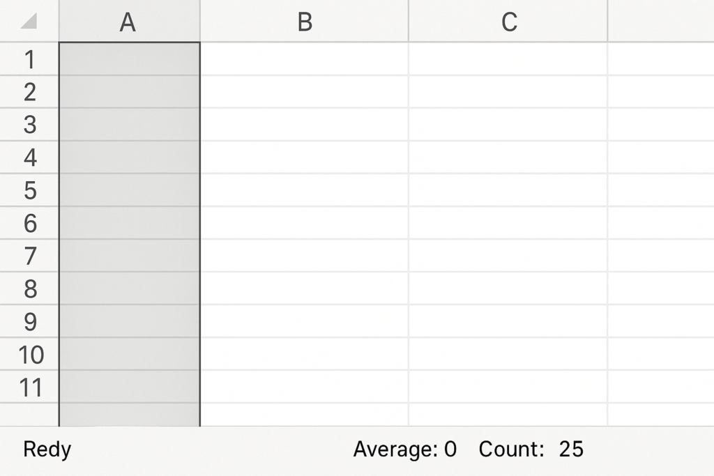
Method 2: Use AutoCalculate in the Status Bar
For quick summaries without formulas:
- Select the column or a range within it.
- Look at the status bar at the bottom of the Excel window.
- It will display basic summaries like Sum, Average, and Count automatically.
This is a fast, no-formula-needed way to understand the data.
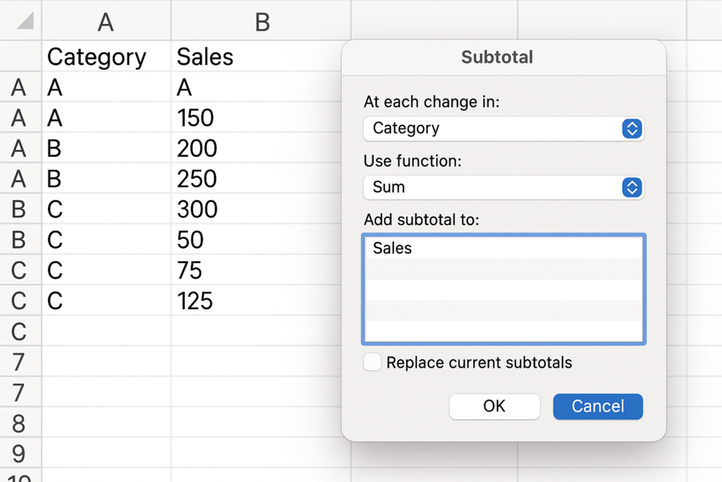
Method 3: Use Subtotal Tool
Excel has a built-in Subtotal feature that summarizes data grouped by a category.
Steps:
- Sort your data based on the category column.
- Go to Data > Subtotal.
- Choose: The column to group by. The function (Sum, Count, Average, etc.) The column you want to summarize.
- Click OK.
This creates an outline where Excel automatically adds summary rows.
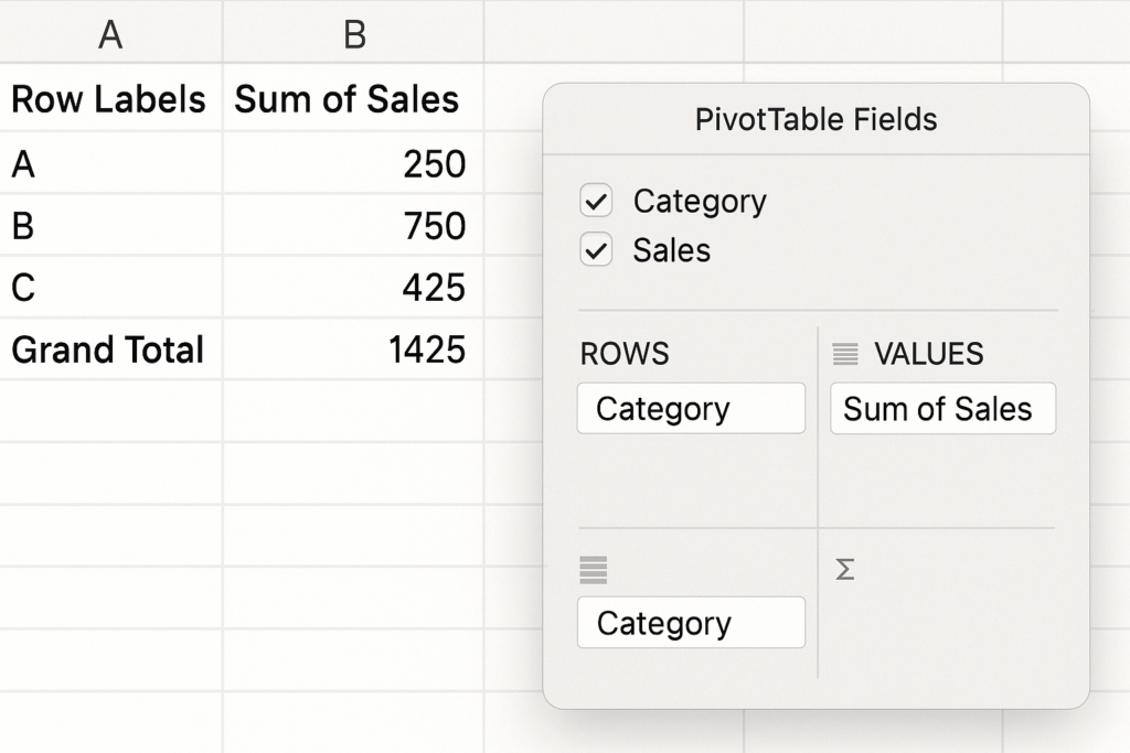
Method 4: Use PivotTable for Advanced Summaries
A PivotTable helps you summarize column data easily. You can filter and group the data as needed.
Steps:
- Select your data range and go to Insert > PivotTable.
- In the PivotTable Fields pane: Drag the column you want to summarize into the Values area. Drag a category or label column into the Rows area if needed.
- Excel will automatically apply a summary function (default is SUM).
You can change the function by clicking the field and selecting Summarize Values By.
Method 5: Use Conditional Summary Functions
If you need to summarize based on conditions, use functions like:
SUMIF
Sum values that meet a specific condition:
=SUMIF(B2:B100, “Completed”, A2:A100)
This adds values in A2:A100 where corresponding cells in B2:B100 are “Completed”.
COUNTIF
Count how many times a condition is met:
=COUNTIF(A2:A100, “>100”)
AVERAGEIF
Get the average of values that meet a condition:
=AVERAGEIF(A2:A100, “>50”)
Examples
Example 1: Sales Summary
You manage a monthly sales log in column D. To calculate the total revenue:
=SUM(D2:D500)
To find the average monthly sale:
=AVERAGE(D2:D500)
Example 2: Attendance Tracking
In column B, you have student names; in column C, “Present” or “Absent.” You can summarize attendance using:
=COUNTIF(C2:C100, “Present”)
Benefits of Summarizing a Column in Excel
Improves Accuracy in Reporting
Formulas reduce the risk of manual errors in calculations. Excel does the math when you use functions or PivotTables. This keeps your insights reliable and consistent.
Helps in Data Validation and Auditing
Summarizing columns can help you spot outliers, missing data, or inconsistencies. If you expect 500 entries but COUNTA shows only 495, that’s a warning sign that some data may be missing.
Supports Dynamic Dashboards and Reports
When used in dashboards, summaries provide real-time metrics that update as data changes. Coupled with data validation or drop-down filters, summaries become interactive and highly functional.
Saves Time in Large-Scale Analysis
For large datasets with thousands of rows, summarization helps reduce complexity. Group and filter key information. This helps stakeholders focus on what truly matters.
Enhances Presentation of Data
Well-summarized data improves the readability and professionalism of reports, presentations, and shared files. Instead of raw tables, decision-makers see polished metrics at a glance.
FAQ’s
Can I summarize filtered data only?
Yes. Use the SUBTOTAL function, which adapts to filtered views:
=SUBTOTAL(109, A2:A100)
This sums only visible rows (109 stands for SUM).
How do I summarize based on categories?
Use a PivotTable or the SUMIF function:
=SUMIF(CategoryRange, “Marketing”, AmountRange)
This adds only the values where the category is “Marketing.”
What’s the fastest way to get basic column summaries?
Select the column and look at the Excel status bar (bottom-right). It shows Sum, Average, and Count instantly without typing a formula.
Can I summarize a column with multiple criteria?
Yes. Use SUMIFS, COUNTIFS, or AVERAGEIFS:
=SUMIFS(AmountRange, CategoryRange, “IT”, StatusRange, “Approved”)
Conclusion
Learning how to summarize a column in Excel is one of the most essential skills for any spreadsheet user. Column summaries help you quickly understand data. They are useful for budgets, task tracking, survey analysis, and dashboard building. Excel provides many options to summarize data. You can use basic functions like SUM and AVERAGE. It also has powerful tools like PivotTables. These summaries save time. They also help with decision-making, data clarity, and reporting accuracy.